The OrthogonalViewer class#

class rockverse.viz.OrthogonalViewer(image, *, region=None, mask=None, segmentation=None, bins=None, ref_voxel=None, ref_point=None, show_xy_plane=True, show_xz_plane=True, show_zy_plane=True, show_histogram=True, show_guide_lines=True, hide_axis=False, image_dict=None, segmentation_alpha=None, segmentation_colors=None, mask_color=None, mask_alpha=None, guide_line_dict=None, histogram_line_dict=None, figure_dict=None, gridspec_dict=None, template='X-ray CT', statusbar_mode='coordinate', layout='2x2', mpi_proc=0)[source]#

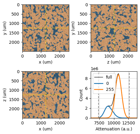
Visualize orthogonal slices (XY, XZ, ZY planes) of a voxel image and its histogram. Supports overlays for masks, segmentations, and region-based filtering.

Parameters:

image (VoxelImage) – The image object to be visualized.
region (Region, optional) – Region object to mask specific voxels on slices and histogram.
mask (VoxelImage, optional) – Boolean voxel image for masking specific voxels on slices and histogram.
segmentation (VoxelImage, optional) – Unsigned int voxel image with segmentation phases to overlay labeled regions on slices and histogram.
bins (int or sequence of scalars, optional) – Binning definition for histogram calculation.
ref_voxel (tuple of int, optional) – Reference voxel (i, j, k) coordinates for slice positioning. Default is the center voxel.
ref_point (tuple of float, optional) – Physical coordinates (x, y, z) in voxel length units, for slice positioning. Overrides ref_voxel.
show_xy_plane (bool, optional) – Display the XY plane slice. Default is True.
show_xz_plane (bool, optional) – Display the XZ plane slice. Default is True.
show_zy_plane (bool, optional) – Display the ZY plane slice. Default is True.
show_histogram (bool, optional) – Display histogram alongside slices. Default is True.
show_guide_lines (bool, optional) – Show guide lines marking slice intersections. Default is True.
hide_axis (bool, optional) – Hide axis labels and ticks in the slice plots. Default is False.
image_dict (dict, optional) – Matplotlib’s AxisImage custom options for image rendering.
segmentation_alpha (float, optional) – Tranparency level for segmentation overlay.
segmentation_colors (str or list, optional) – A string representing a predefined colormap or a list of colors. If a string, it should be the name of a Matplotlib qualitative colormap (e.g., ‘Set1’, ‘Pastel1’, ‘Pastel1_r’). If a list, it should contain colors in a format acceptable by Matplotlib (e.g., RGB tuples, hex codes). The colors will be cycled through and assigned to the segmentation phases.
mask_color (Any, optional) – Color for mask overlay. Any color format accepted by Matplotlib.
mask_alpha (float, optional) – Tranparency level for mask overlay. It must be a float between 0.0 and 1.0.
guide_line_dict (dict, optional) – Matplotlib’s Line2D custom options for guide lines (e.g., linestyle, color, linewidth).

histogram_line_dict (dict, optional) –

Custom options for Matplotlib’s Line2D in the histogram plot.

This dictionary must include the following structure:

{
    'full': <**kwargs>,   # For the full histogram
    'phases': <**kwargs>, # For segmentation phases
    'clim': <**kwargs>    # For the vertical CLIM lines
}

Example:

histogram_line_dict = {
    'full': {'color': 'blue', 'linewidth': 2},
    'phases': {'linestyle': '--', 'alpha': 0.7},
    'clim': {'color': 'red', 'linewidth': 1}
}

figure_dict (dict, optional) – A Dictionary of keyword arguments to be passed to the underlying Matplotlib figure creation.
gridspec_dict (dict, optional) – Dictionary of keyword arguments for customizing the grid layout of the figure, generated using Matplotlib gridspec. Width and height ratios are automatically calculated from image dimensions.
template ({'X-ray CT', 'Scalar field'}, optional) –
The template to use for visualizing the orthogonal slices. This parameter determines the default settings for the viewer, including colormaps, alpha values, and other rendering options. Note that values from templates have lower precedence than other customization parameters.

Available templates:
- ’X-ray CT’: the default value, optimized for X-ray computed tomography images, with settings suitable for visualizing attenuation values.
- ’Scalar field’: optimized for scalar fields such as electric potentials or velocity components.
statusbar_mode ({'coordinate', 'index'}) –
The desired status bar information mode when hovering the mouse over the figure in interactive mode:
- ’coordinate’ for physical coordinates.
- ’index’ for voxel indices.
layout ({'2x2', 'vertical', 'horizontal'}, optional) –
The layout configuration for displaying the orthogonal slices and histogram.

This parameter determines how the various components (XY, XZ, ZY slices, and histogram) are arranged within the figure. The following layout options are available:
- ’2x2’: Arranges the XY and ZY slices in the top row and the XZ slice and histogram in the bottom row, creating a 2x2 grid layout.
- ’vertical’: Stacks the XY, ZY, XZ, and XZ slices vertically in a single column, and places the histogram below them.
- ’horizontal’: Places the XY slice on the left, followed by the ZY slice, the XZ slice, and the histogram plot.
The default layout is ‘2x2’. This parameter allows for flexible visualization of the slices and histogram based on user preferences or specific analysis needs.
mpi_proc (int, optional) – MPI process rank responsible for figure rendering. Default is 0.

Returns:

The OrthogonalViewer instance.

Return type:

OrthogonalViewer

Matplotlib-related attributes

`figure`	The Matplotlib Figure object.
`ax_xy`	The Matplotlib Axes object for the xy slice.
`ax_zy`	The Matplotlib Axes object for the zy slice.
`ax_xz`	The Matplotlib Axes object for the xz slice.
`ax_histogram`	The Matplotlib Axes object for the histogram plot.

RockVerse objects

`image`	The input image data.
`region`	Get or set the region of interest.
`mask`	Get or set the mask image.
`segmentation`	Get or set the segmentation image.
`histogram`	The `rockverse.Histogram` object.

Axes building attributes

`show_xy_plane`	Boolean flag to enable or disable the visibility of the XY slice.
`show_xz_plane`	Boolean flag to enable or disable the visibility of the XZ slice.
`show_zy_plane`	Boolean flag to enable or disable the visibility of the ZY slice.
`show_histogram`	Boolean flag to enable or disable the visibility of the histogram plot.
`gridspec_dict`	Dictionary of keyword arguments for customizing the figure's grid layout.
`update_gridspec_dict`(**kwargs)	Update the gridspec settings dictionary and rebuilds the display.
`layout`	Get or set the figure grid layout.

View customization attributes and methods

`ref_voxel`	Get or set the plot reference point in voxel position.
`ref_point`	Get or set the plot reference point in voxel units.
`image_dict`	Get the dictionary of keyword arguments for customizing the image display.
`update_image_dict`(**kwargs)	Update the image display settings dictionary and refreshes the display.
`show_guide_lines`	Boolean flag to enable or disable the visibility of the guide lines for slice intersection.
`guide_line_dict`	Get the dictionary of Matplotlib's `Line2D` keyword arguments used for customizing the guide lines.
`update_guide_line_dict`(**kwargs)	Update the guide line display settings dictionary and refresh the display.
`segmentation_colors`	Get or set the color list for the segmentation phases.
`segmentation_colormap`	Get the segmentation colorlist as a Matplotlib colormap.
`segmentation_alpha`	Get or set the transparency level for segmentation overlay.
`mask_color`	Get or set the color for the mask overlay.
`mask_alpha`	Get or set the transparency level for the mask overlay.
`histogram_bins`	Get or set the histogram bins.
`histogram_line_dict`	Get the dictionary of keyword arguments for customizing the histogram lines.
`update_histogram_line_dict`(v)	Update the histogram lines display settings dictionary and refreshes the display.
`histogram_lines`	A dictionary with the Matplotlib `Line2D` for each line in the histogram plot.
`hide_axis`	Boolean flag to control the visibility of image axes and labels.
`shrink_to_fit`()	Adjust the figure size to fit the ideal proportions of the content.
`expand_to_fit`()	Adjust the figure size to ensure that all content fits within the figure.
`statusbar_mode`	Get or set the status bar display mode.

figure#: The Matplotlib Figure object.

ax_xy#: The Matplotlib Axes object for the xy slice.

ax_zy#: The Matplotlib Axes object for the zy slice.

ax_xz#: The Matplotlib Axes object for the xz slice.

ax_histogram#: The Matplotlib Axes object for the histogram plot.

image#: The input image data.

region#

Get or set the region of interest.

Examples

>>> from rockverse.regions import Cylinder
>>> viewer = rockverse.OrthogonalViewer(<your parameters here...>)
>>> viewer.region = Cylinder(<your parameters here...>)  # Set a new region
>>> region = viewer.region                               # Get the current region
>>> viewer.region = None                                 # Remove the region

mask#

Get or set the mask image.

Examples

>>> viewer = rockverse.OrthogonalViewer(<your parameters here...>)
>>> mask = viewer.mask            # Get the current mask
>>> viewer.mask = new_mask_image  # Set a new voxel image as mask
>>> viewer.mask = None            # Remove the mask

segmentation#

Get or set the segmentation image.

Examples

>>> viewer = rockverse.OrthogonalViewer(<your parameters here...>)
>>> segmentation = viewer.segmentation     # Get the current segmentation image
>>> viewer.segmentation = new_segmentation # Set a new image for segmentation
>>> viewer.segmentation = None             # Remove the segmentation

histogram#: The rockverse.Histogram object.

show_xy_plane#

Boolean flag to enable or disable the visibility of the XY slice.

When set to True, the XY slice will be displayed in the viewer. When set to False, the XY slice will be hidden. Changing this setting will rebuild the visualization to reflect the current state.

Examples

>>> viewer.show_xy_plane          # Get the current state
>>> viewer.show_xy_plane = True   # Show the XY slice
>>> viewer.show_xy_plane = False  # Hide the XY slice

show_xz_plane#

Boolean flag to enable or disable the visibility of the XZ slice.

When set to True, the XZ slice will be displayed in the viewer. When set to False, the XZ slice will be hidden. Changing this setting will rebuild the visualization to reflect the current state.

Examples

>>> viewer.show_xz_plane          # Get the current state
>>> viewer.show_xz_plane = True   # Show the XZ slice
>>> viewer.show_xz_plane = False  # Hide the XZ slice

show_zy_plane#

Boolean flag to enable or disable the visibility of the ZY slice.

When set to True, the ZY slice will be displayed in the viewer. When set to False, the ZY slice will be hidden. Changing this setting will rebuild the visualization to reflect the current state.

Examples

>>> viewer.show_zy_plane          # Get the current state
>>> viewer.show_zy_plane = True   # Show the ZY slice
>>> viewer.show_zy_plane = False  # Hide the ZY slice

show_histogram#

Boolean flag to enable or disable the visibility of the histogram plot.

Examples

>>> viewer.show_histogram         # Get the current visibility state of the histogram
>>> viewer.show_histogram = True  # Show the histogram
>>> viewer.show_histogram = False # Hide the histogram

gridspec_dict#

Dictionary of keyword arguments for customizing the figure’s grid layout.

This dictionary is passed to Matplotlib’s GridSpec when creating the figure layout. It can be used to control aspects such as spacing between subplots. Width and height ratios are automatically calculated from image dimensions. See the documentation for Matplotlib GridSpec.

Important: Do not change elements directly in this dictionary. Call the update_gridspec_dict method instead to apply any changes.

update_gridspec_dict(**kwargs)[source]#

Update the gridspec settings dictionary and rebuilds the display. See the documentation for the gridspec_dict method.

Examples

>>> viewer.update_gridspec_dict(width_ratios=[1, 4])  # Update width ratios

layout#

Get or set the figure grid layout. Allowed values are:

‘2x2’: Arranges the XY and ZY slices in the top row and the XZ slice and histogram in the bottom row, creating a 2x2 grid layout.
‘vertical’: Stacks the XY, XZ, and ZY slices vertically in a single column, and places the histogram below them.
‘horizontal’: Places the XY slice on the left, the ZY slice in the middle, and the XZ slice on the right, with the histogram below.

The default layout is ‘2x2’. This parameter allows for flexible visualization of the slices and histogram based on user preferences or specific analysis needs.

Examples

>>> layout = viewer.layout      #Get the current layout state
>>> viewer.layout = 'vertical'  #Set the grid layout to vertical mode

ref_voxel#

Get or set the plot reference point in voxel position. Voxel position must be an iterable (i, j, k), where 0 <= i < nx, 0 <= j < ny, and 0 <= k < nz, with nx, ny, nz = image.shape.

Examples

>>> viewer = rockverse.OrthogonalViewer(<your parameters here...>)
>>> ref_voxel = viewer.ref_voxel #get the current reference voxel
>>> viewer.ref_voxel = (8, 33, 9) # Set new reference voxel and update

ref_point#

Get or set the plot reference point in voxel units.

Get or set the plot reference point in image position. It must be an ordered iterable (x, y, z), where ox <= x < ox+hx*nx, oy <= y < oy+hy*ny, and oz <= z < oz+hz*nz, with ox, oy, oz = image.voxel_origin, hx, hy, hz = image.voxel_length, and nx, ny, nz = image.shape. If (x, y, z) is not a grid point, the closest grid point will be used.

Examples

>>> viewer = rockverse.OrthogonalViewer(<your parameters here...>)
>>> ref_point = viewer.ref_voxel #get the current reference voxel
>>> viewer.ref_point = (3.33, 14.72, 10) # Set new reference point and update

image_dict#

Get the dictionary of keyword arguments for customizing the image display.

This dictionary is passed to Matplotlib’s imshow function when displaying the image slices. It can be used to control aspects such as colormap, alpha (transparency), etc. See the documentation for Matplotlib imshow function.

Important: Do not change elements directly in this dictionary. Call the update_image_dict method instead to apply any changes.

update_image_dict(**kwargs)[source]#

Update the image display settings dictionary and refreshes the display. See the documentation for the image_dict property.

Example

>>> # Update colormap and transparency
>>> viewer.update_image_dict(cmap='gray', alpha=0.8)

show_guide_lines#

Boolean flag to enable or disable the visibility of the guide lines for slice intersection.

Examples

>>> viewer.show_guide_lines         # Get the current visibility state
>>> viewer.show_guide_lines = True  # Show the guide lines
>>> viewer.show_guide_lines = False # Hide the guide lines

guide_line_dict#

Get the dictionary of Matplotlib’s Line2D keyword arguments used for customizing the guide lines.

Important: Do not change elements directly in this dictionary. Call the update_guide_line_dict method instead to apply any changes.

update_guide_line_dict(**kwargs)[source]#

Update the guide line display settings dictionary and refresh the display.

This method allows you to modify the settings in the guide_line_dict that control the appearance of the guide lines drawn on the image slices. You can update various parameters by passing the desired keyword arguments.

Examples

>>> # Update guide lines to be red, dashed, and with a width of 2
>>> viewer.update_guide_line_dict(color='red', linestyle='--', linewidth=2)

segmentation_colors#

Get or set the color list for the segmentation phases.

If a string, it should be the name of a predefined Matplotlib qualitative colormap (e.g., ‘Set1’, ‘Pastel1’, ‘Pastel1_r’).
If a list, it should contain colors in any format acceptable by Matplotlib, such as RGB tuples (e.g., (1, 0, 0) for red), hex codes (e.g., ‘#FF0000’ for red), or named colors (‘gold’, ‘forestgreen’, etc.).

The specified colors will be cycled through and assigned to the segmentation phases.

Examples

>>> viewer.segmentation_colors = 'tab10'  # Using a predefined Matplotlib colormap
>>> viewer.segmentation_colors = [(1, 0, 0), '#339966', 'gold']  # Using a list with any valid format

segmentation_colormap#: Get the segmentation colorlist as a Matplotlib colormap.

segmentation_alpha#

Get or set the transparency level for segmentation overlay. The value must be a float between 0.0 and 1.0, where 0.0 is fully transparent (invisible) and 1.0 is fully opaque (completely visible).

Examples

>>> viewer.segmentation_alpha = 0.5            # Set the transparency to 50%
>>> current_alpha = viewer.segmentation_alpha  # Get the current transparency level

mask_color#

Get or set the color for the mask overlay.

This property defines the color used for the mask overlay displayed on the image slices. The color can be specified in any format accepted by Matplotlib, including named colors (e.g., ‘red’, ‘blue’, ‘royalblue’), RGB tuples (e.g., (1, 0, 0) for red), or hex codes (e.g., ‘#00FF00’ for green).

The chosen color will be used to visually indicate masked areas on the image.

Examples

>>> current_color = viewer.mask_color           # Get the current mask color
>>> viewer.mask_color = 'white'                 # Set the mask color to white
>>> viewer.mask_color = (0.25, 0.30, 0.25)      # Set the mask color using an RGB tuple
>>> viewer.mask_color = '#008000'               # Set the mask color using a hex code

mask_alpha#

Get or set the transparency level for the mask overlay.

This property controls the alpha (transparency) value of the mask overlay displayed on the image slices. The value must be a float between 0.0 and 1.0, where 0.0 is fully transparent (invisible) and 1.0 is fully opaque (completely visible).

Examples

>>> viewer.mask_alpha = 0.5   # Set the transparency to 50%
>>> current_alpha = viewer.mask_alpha  # Get the current transparency level

histogram_bins#: Get or set the histogram bins.

histogram_line_dict#

Get the dictionary of keyword arguments for customizing the histogram lines.

Important: Do not change elements directly in this dictionary. Call the update_image_dict method instead to apply any changes.

update_histogram_line_dict(v)[source]#

Update the histogram lines display settings dictionary and refreshes the display. Value must be a dictionary with the following structure:

{
    'full': <**kwargs>,   # For the full histogram
    'phases': <**kwargs>, # For segmentation phases
    'clim': <**kwargs>    # For the vertical CLIM lines
}

Examples:

viewer.update_histogram_line_dict({
    'full': {'color': 'blue', 'linewidth': 2},
    'phases': {'linestyle': '--', 'alpha': 0.7},
    'clim': {'color': 'red', 'linewidth': 1}
})

You can use only a subset of the keywords:

viewer.update_histogram_line_dict({
    'phases': {'linestyle': '--'}})

histogram_lines#: A dictionary with the Matplotlib Line2D for each line in the histogram plot.

hide_axis#

Boolean flag to control the visibility of image axes and labels.

When set to True, the axes and labels for the image slices will not be drawn, providing a cleaner visual presentation that focuses solely on the image data. This can be useful in cases where the axes are not needed for interpretation or when a more aesthetic visualization is desired. The default value is False.

Examples

>>> viewer.hide_axis         # Get the current visibility state of the axes
>>> viewer.hide_axis = True  # Hide the axes and labels
>>> viewer.hide_axis = False # Show the axes and labels

shrink_to_fit()[source]#

Adjust the figure size to fit the ideal proportions of the content.

This method reduces the size of the figure by scaling down the largest side to ensure that all axes and components fit neatly within the figure without unnecessary white space. It helps optimize the layout of the visualization, particularly after modifications to the displayed planes or components.

This method is especially useful when toggling the visibility of different slices or adjusting the figure’s contents, ensuring that the presentation remains visually appealing and focused on the data.

expand_to_fit()[source]#

Adjust the figure size to ensure that all content fits within the figure.

This method increases the size of the figure by scaling up the smallest side to match the ideal proportions of the displayed content. It ensures that all axes, components, and visual elements are adequately visible without clipping or unnecessary overlap.

This method is particularly useful after changing which planes or components are displayed, helping to maintain an optimized layout and providing a more comprehensive view of the data.

statusbar_mode#

Get or set the status bar display mode.

This property determines the information displayed in the status bar when hovering the mouse over the figure in insteractive mode. It can show either the physical coordinates of the cursor position or the voxel indices of the corresponding data point.

Available modes:

‘coordinate’: displays the physical coordinates (x, y, z) in the current units of the image.
‘index’: displays the voxel indices (i, j, k) corresponding to the cursor position in the voxel grid.

Examples

>>> viewer.statusbar_mode                 # Get the current mode
>>> viewer.statusbar_mode = 'coordinate'  # Set status bar to show physical coordinates
>>> viewer.statusbar_mode = 'index'       # Set status bar to show voxel indices

Interactive Features#

The OrthogonalViewer class offers interactive features that enhance the user experience by allowing real-time updates and interactions with the visualized data, including the displayed slices and histograms.

Note

To utilize the interactive features, ensure that Matplotlib is configured for interactive mode. You can use backends such as Qt5Agg or ipympl for Jupyter Notebooks.

Users can interact with the visualization through mouse actions on the image slices or the histogram. The following actions are supported:

Left click on image slices: Displays voxel data at the cursor position in the console.
Right click on image slices: Updates the reference point to the cursor position, allowing users to change the displayed slices.
Middle click on image slices: Resets the reference point to the center of the image bounding box.
Left click on the histogram: Sets the image minimum color limit (clim) value to the horizontal coordinate of the click.
Right click on the histogram: Sets the image maximum color limit (clim) value to the horizontal coordinate of the click.
Middle click on the histogram: Resets the image color limit (clim) values to the 99.9% confidence interval based on the histogram data.

The OrthogonalViewer class#

Interactive Features#

Related tutorials#

This Page