Importing the C04B21 dataset

The data for our tutorial on processing dual energy X-ray computed tomography (CT) is the C04B21 carbonate core CT dataset. This dataset is part of a collection of dual energy medical CT scans of 3 ft carbonate core samples, made available by Rodolfo Victor at the Digital Rocks Portal. The scans were acquired with a voxel size of (0.488 X 0.488 X 1.25) mm at the Petrobras Research Center.

The C04B21 dataset represents a carbonate core sample imaged using dual-energy CT, which provides valuable information about the sample’s internal structure and composition. We will use this data to demonstrate the processing and analysis capabilities of RockVerse.

Note

If you plan to use this data, please remember to cite the data and the related publications.

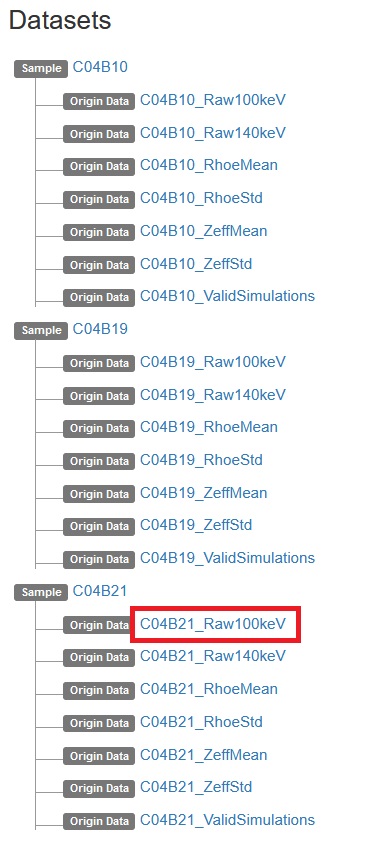
To download the data, visit the Dual-energy medical CT in carbonate rocks project on the Digital Rocks Portal: https://www.digitalrocksportal.org/projects/102. Click on the low-energy image C04B21_Raw100keV.

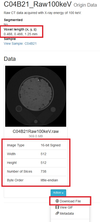
Pay attention to the metadata, as we will need this information later in the tutorial. Note that this is ImageJ/Fiji exported raw data, so it is in Fortran file order. Click Action->Download File.

Repeat the procedure and download the high-energy image C04B21_Raw140keV.

Now, let’s import the raw files into RockVerse. In this example, we’ll use 8 chunks by halving the number of voxels in each direction:

import rockverse as rv

# Importing low energy raw image as a RockVerse voxel image
C04B21_Raw100keV =  rv.voxel_image.import_raw(
    rawfile='/path/to/rawdata/dual_energy_carbonate/C04B21Raw100keV.raw',
    raw_file_order='F',                  #<- Raw file is in Fortran file order
    store='/path/to/imported/dual_energy_carbonate/C04B21Raw100keV',
    shape=(512, 512, 738),               #<- From metadata, image size (nx, ny, nz)
    chunks=(256, 256, 369),              #<- Our choice of chunk size. Will give a 2x2x2 chunk grid
    dtype='<i2',                         #<- From metadata, little-endian 16-bit signed integer
    offset=0,                            #<- From metadata
    voxel_length=(0.488, 0.488, 1.25),   #<- From metadata
    voxel_unit='mm',                     #<- From metadata
    field_name='Low energy attenuation', #<- Our choice for field name (X-ray attenuation)
    field_unit='H.U.',                   #<- field units (Hounsfield units)
    description='Low energy X-ray CT attenuation', #<- General data description
    overwrite=True                       #<- Overwrite if file exists in disk
    )

# Importing high energy raw image as a RockVerse voxel image
C04B21_Raw140keV =  rv.voxel_image.import_raw(
    rawfile='/path/to/rawdata/dual_energy_carbonate/C04B21Raw140keV.raw',
    raw_file_order='F',
    store='/path/to/imported/dual_energy_carbonate/C04B21Raw140keV',
    shape=(512, 512, 738),
    chunks=(256, 256, 369),
    dtype='<i2',
    offset=0,
    voxel_length=(0.488, 0.488, 1.25),
    voxel_unit='mm',
    field_name='High energy attenuation',
    field_unit='H.U.',
    description='High energy X-ray CT attenuation',
    overwrite=True
    )

[2025-02-25 11:14:51] (Low energy attenuation) Importing raw file: 100%|>>>>>>>>>>| 8/8 [00:08<00:00,  1.05s/chunk]
[2025-02-25 11:14:59] (High energy attenuation) Importing raw file: 100%|>>>>>>>>>>| 8/8 [00:08<00:00,  1.08s/chunk]

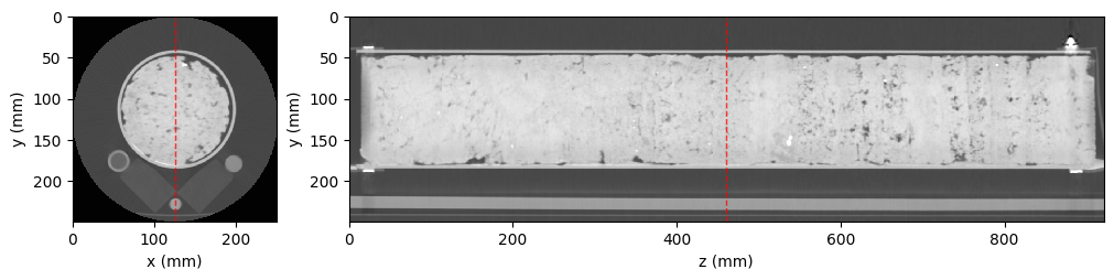
The images are now available as RockVerse voxel images on disk, at the path specified in the store parameter. Let’s do a quick visualization using RockVerse’s orthogonal viewer:

# Create an OrthogonalViewer for the low-energy image
lowE_viewer = rv.OrthogonalViewer(C04B21_Raw100keV,
                                 show_xz_plane=False,
                                 show_histogram=False,
                                 )

# Create an OrthogonalViewer for the high-energy image
highE_viewer = rv.OrthogonalViewer(C04B21_Raw140keV,
                                 show_xz_plane=False,
                                 show_histogram=False,
                                 )

# The Matplotlib figure object is available through the viewer figure property
lowE_viewer.figure.set_size_inches(10, 10)
highE_viewer.figure.set_size_inches(10, 10)

[2025-02-25 11:24:43] Histogram Low energy attenuation (min/max): 100%|>>>>>>>>>>| 8/8 [00:01<00:00,  6.16chunk/s]
[2025-02-25 11:24:44] Histogram Low energy attenuation (counting voxels): 100%|>>>>>>>>>>| 8/8 [00:05<00:00,  1.54chunk/s]
[2025-02-25 11:24:53] Histogram High energy attenuation (min/max): 100%|>>>>>>>>>>| 8/8 [00:01<00:00,  6.26chunk/s]
[2025-02-25 11:24:54] Histogram High energy attenuation (counting voxels): 100%|>>>>>>>>>>| 8/8 [00:05<00:00,  1.59chunk/s]

Now that we have successfully imported the raw images, we can move on to the next part of this tutorial.